Then the initial condition u(x, 0) = f I will appreciate if i can get the code and lectures on how to write or a comprehensive code and how to modify.
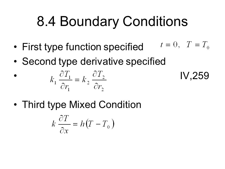
Differential Equations Modeling With Higher Order Linear De Boundary Value Problems
Using boundary conditions, write, n*m equations for u(x i=1:m,y j=1:n) or n*m unknowns.

How to solve differential equations with boundary conditions. How to the scipy solve_ivp function to integrate first oder odes in python.the 'ivp' stands for initial value problem which means it can be used to solve problems where we know all the boundary conditions at a single point in space or time.solve_ivp is designed to trivially solve first order odes, other videos will show how to solve harder problems. We will apply separation of variables to each problem and find a product solution that will satisfy the differential equation and the three homogeneous boundary conditions. The equation in question is a coupled nonlinear ode with boundary conditions.
Therefore, the only particular solution for these particular boundary conditions is y ( x) = 0, the trivial solution. For instance, for a second order differential equation the initial conditions are, y(t0) = y0 y′(t0) = y′ 0 y ( t 0) = y 0 y ′ ( t 0) = y 0 ′. So you need to solve the system of equations $$x = \frac{s^2}{2}+x_0$$ $$y = s + x_0^2$$
Iterating $n$ times introduces $n$ constants.) to find these parameters, you need $n$ conditions, which can involve the function and/or its derivatives at some points. Recall that we had solved such nonhomogeneous differential equations in chapter 2. F''(t) = 3*f(t)*g(t) + 5 g''(t) = 4*g(t)*f(t) + 7 with initial conditions:
Partial differential equations with boundary conditions significant developments happened for maple 2019 in its ability for the exact solving of pde with boundary / initial conditions. You do have a boundary condition, it is $u=0$ on the parabola $y=x^2$. Considering the same problem i'm assuming the equations to be solved are:
The new functionality is described below, in 11 brief sections, with 30 selected examples and a few comments. In[16]:= eqns = 8f''@xd == g@xd, f@xd + g@xd == 3 sin@xd, f@pid == 1, f'@pid == 0<; Then, equation (4.1) takes the form ly = f.
In this chapter we will learn how to solve ode boundary value problem. 3 = 0 → a = 0. $y'' [x] = {k^2}y [x]$.
To finish the problem, you need to find for a given point $(x,y)$ in the plane which characteristic curve passes through that point, and the value of $s$ at which it exactly hits $(x,y)$. Y ′ ( 0) = 0; Y p(x) y q(x) y f(x) a x b (1a) and the boundary conditions (bc) are given at both end of the domain e.g.
(taking an antiderivative introduces an integration constant; Y ( 1) = 0. Let’s change the question and ask ourselves now if there is any number λ, so that the equation.
Using a substitution to help us solve differential equations. Not all boundary conditions allow for solutions, but usually the physics suggests what makes sense. Find the fourier series solution to the differential equation \[y^{\prime\prime} + 2y = 3x\] with the boundary conditions \(y\left( 0 \right) = y\left( 1 \right) = 0.\) solution.
F(0) = 1.5, g'(0) = 0 and boundary constraints defined at tf = 1: We can write such an equation in operator form by defining the differential operator l = a2(x)d2 + a1(x)d + a0(x), where d = d/dx. Bv ode is usually given with x being the independent space variable.
The general solution of an $n^{th}$ order differential equation depends on $n$ unknown parameters. I1,j i,j i1,j2 2 22 u2uu x o( x ) u x() −+−+ δ δ ∂ ∂ =+ 22 2 22 2 uuuu uu4u i 1,j i 1,j i,j 1 i,j 1 i,j o(h ) xy h ∂∂−+ −+++ +− ∂∂ += + i,j 1 i,j i,j 1 2 2 With boundary value problems we will have a differential equation and we will specify the function and/or derivatives at different points, which we’ll call boundary values.
Y ″ ( x) + λ y ( x) = 0; The general solution (that satisfies the boundary conditions) shall be solved from this system of simultaneous differential equations. X ″ + λx = 0, x(0) = 0 and x(l) = 0, t ′ + α 2 λ t = 0.
Y(a) = and y(b) =. In this section we will show that these equations can be solved The syntax is the same as for a system of ordinary differential equations.
Dear friends, i am going to solve the following differential equation: Equations, together with a set of two boundary conditions that go with the equation of the spatial variable x: So these are uncoupled for now, and pretty straightforward to solve.
You can solve by putting all types of boundary conditions in fem.first of all you discretise the boundary in such a way that your global stiffness matrix will be symmetric and diagonal dependent. We first solve the equation with the boundary condition (b.c.) at 0 i.e. Solve this banded system with an efficient scheme.
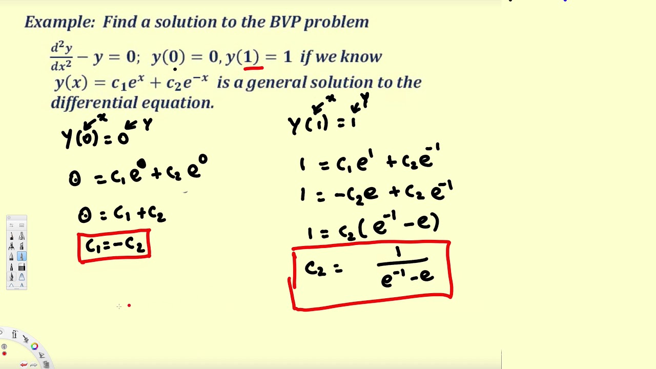
Using the principle of superposition we’ll find a solution to the problem and then apply the final boundary condition to determine the value of the constant(s) that are left in the problem. The boundary conditions are passed to dsolve as a dictionary, through the ics named argument. G(1) = 3, f'(1) =q* f(1)
We will use the fourier sine series for representation of the nonhomogeneous solution to satisfy the boundary conditions. Let me remind you of the situation for ordinary differential equations, one you should all be familiar with, a particle under the influence of a constant force,
Boyces Elementary Differential Equations And Boundary Value Problems 11th Edition Global Edition Wiley

Boundary Value Problems And Partial Differential Equations Pdes - Ppt Video Online Download

Solutions Manual For Differential Equations Computing And Modeling And Differential Equations And Boundary V Differential Equations Equations Algebra Problems

Intro To Boundary Value Problems - Differential Equations 1 Differential Equations Equations Problem

Intro Boundary Value Problems 2 - Differential Equations Differential Equations Equations Intro
S2pnd-matematikafkipunpattiacid
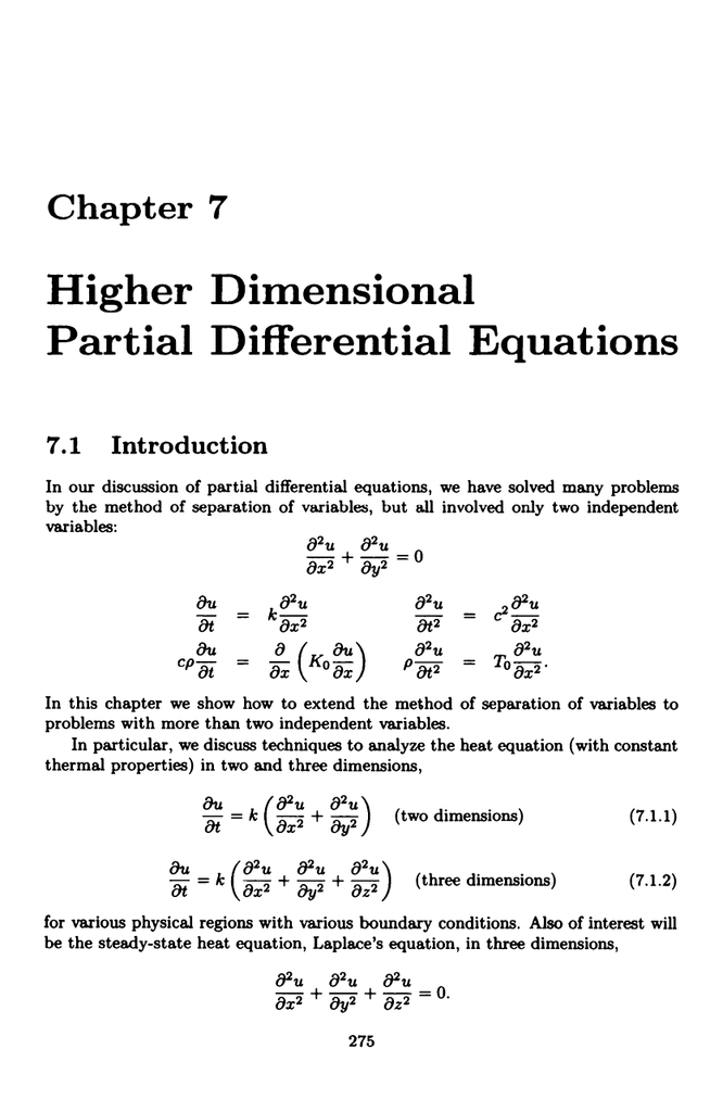
Partial Differential Equations Higher Dimensional Chapter 7 Introduction

Differential Equations With Boundary-value Problems Dennis G Zill Warren S Wright Good And Easy Book To Elemen Differential Equations Equations Textbook

Partial Differential Equations Boundary Value Problems With Maple Sciencedirect
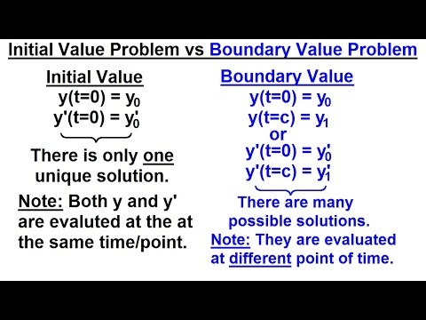
Differential Equation - 2nd Order 29 Of 54 Initial Value Problem Vs Boundary Value Problem - Youtube

Boundary Value Problems And Partial Differential Equations Pdes - Ppt Video Online Download

Elementary Differential Equations And Boundary Value Problems Edition 11th Ebook Pdf Marketingebook Ebookpdf Differential Equations Equations Math Textbook

Boycediprima 10th Ed Ch 101 Two-point Boundary Value Problems Elementary Differential Equations And Boundary Value Problems 10th Edition By William - Ppt Video Online Download

Boundary Value Problems And Partial Differential Equations Pdes - Ppt Video Online Download
Chapter 8 Partial Differential Equation 81 Introduction Independent Variables Formulation Boundary Conditions Compounding Method Of Image Separation - Ppt Download
Robot Check Differential Equations Equations Elementary

Pin On Solutions Manual
Classification

Intro To Boundary Value Problems - Differential Equations 1 - Youtube